Ama Dablam: A 322M Linear/Dense Hybrid Language Model for Nepali, Maithili, and Bhojpuri Across Three Writing Systems

Abstract

We present Ama Dablam, a 322-million-parameter decoder-only language model pretrained from scratch on Nepali, Maithili, and Bhojpuri rendered in three writing systems: native Devanagari, scholarly IAST romanization, and natural (“speaker-style”) phonetic romanization. The model achieves a bits-per-byte (bpb) of 0.4061 on a pinned held-out Nepali shard, surpassing our earlier, internal 491M dense model (0.4324) on every language, an outcome anticipated by a scaling law fitted on runs 592× smaller and driven by training volume (3.6× more tokens) rather than parameter count. We make three contributions. First, a phonetic corpus-augmentation pipeline: a deterministic Devanagari→Latin transliterator implementing Nepali schwa deletion, which produces romanized training text from existing Devanagari data at zero collection cost. Second, a linear/dense hybrid attention architecture that interleaves 12 linear-attention layers with 2 softmax layers, trained at 17.1B-token scale with the full tuning history including negative results. Its linear layers use RetNet-style [1] per-head exponential decay, meaning each head discounts a token \(j\) positions back by a factor \(\gamma^{\,j}\), with every head assigned its own \(\gamma\), so that one layer spans memory horizons ranging from a few tokens to the whole document. Third, multi-script instruction tuning, in which a content-hash-partitioned SFT dataset (85% Devanagari / 5% IAST / 10% phonetic) plus a 5% pretraining-replay stream yields a model that follows instructions in whichever script it is addressed, improving response-level bpb by 31–40% in every script while limiting catastrophic forgetting [2] on all replay-covered evaluation sets to ≤ +0.04 bpb.

---

1. Introduction

Nepali (approx 16–32M speakers), Maithili (approx 17–34M), and Bhojpuri (approx 50–52M) are together spoken by on the order of a hundred million people [3, 4], yet remain severely underserved by language technology. Frontier multilingual models tokenize Devanagari at substantially higher cost than English, often 2× or more in token length for the same content [5]. They dilute these languages to tiny fractions of their training mix [4, 6], and for Maithili and Bhojpuri they remain weak on the few benchmarks that exist (e.g., Gemini-2.5, the strongest model evaluated, reaches only 54% on IndicParam Maithili MCQs and under 60% average across the suite) [4]. At the same time, speakers of these languages routinely write them in Latin script on phones and social media [7], an input mode almost no model handles.

This report documents a complete, reproducible campaign covering corpus construction, tokenizer, architecture, pretraining, evaluation, and instruction tuning, executed on a single NVIDIA DGX Spark (GB10) workstation. Throughout, the measured baseline is our earlier 491M dense model, trained earlier in the same campaign (4.8B tokens) on the same corpus lineage under the same frozen evaluation protocol, though on a smaller corpus without phonetic augmentation; its configuration is summarized in Appendix E so that this report is self-contained.

Contributions.

1. Phonetic corpus augmentation for Devanagari languages (§2.3). A deterministic transliterator implementing natural Nepali romanization (schwa deletion, aspirate digraphs, homorganic nasal resolution) converts existing Devanagari text into Latin script the way speakers actually type it. Applied to 10% of the Nepali corpus and 100% of Maithili/Bhojpuri, it adds a third writing system to the model’s competence at zero data-collection cost.
2. A linear/dense hybrid at scale, with its tuning history (§4–5). Twelve of fourteen layers use O(T) linear attention with per-head exponential decay (base γ = 0.7, the single knob that made linear attention [8] competitive); two use full softmax. We report the small-scale tuning evidence, including the equal-FLOPs vs equal-tokens accounting trap and the absence of a matched dense baseline at production scale.
3. Multi-script instruction tuning with replay-based script preservation (§8). Instruction data partitioned by content hash into 85/5/10 Devanagari/IAST/phonetic slices (whole example, one script), plus a 5% replay stream drawn from the pretraining shards in their native mix, produces script-following behavior (reply in the script you are addressed in) while bounding forgetting on every replay-covered metric.
4. Practical takeaways (§10) and a forward agenda (§11), each tied to a measured number from this campaign.

Headline results.

Metric	Earlier 491M dense	Ama Dablam (322M hybrid)
val_bpb Nepali (shard 06542)	0.4324	0.4061 (−6.1%)
val_bpb Maithili (06543)	0.4383	0.3677 (−16.1%)
val_bpb Bhojpuri (06544)	0.6320	0.5461 (−13.6%)
Pretraining tokens	~4.8B (9.8 tok/param)	17.1B (53.1 tok/param)
Parameters	490.7M	321.8M
SFT response-bpb (overall)	n/a	0.5696 → 0.3471 (−39%)

---

2. Corpus Construction and Curation

2.1 Base trilingual corpus

By trilingual corpus we mean one pooled training set that mixes all three languages together, rather than three separate per-language corpora feeding three separate models. Nepali, Maithili, and Bhojpuri are closely related Indo-Aryan languages that share the Devanagari script, so one model can serve all three, and the two smaller languages benefit from patterns learned on the largest (§10, item 4). What controls each language’s influence is therefore its share of the mixture, set in the mixing step below.

This Devanagari base corpus is inherited from the data pipeline that trained the earlier 491M dense model (Appendix E); we summarize below the facts needed to make this report self-contained.

Sources. Nepali: iriis_nepali_corpus and original_pretrain (local), ai4bharat/sangraha [9] (verified/nep), wikimedia/wikipedia [10] (20231101.ne), spandyie/nepali-news-dataset. Maithili: sangraha (verified/mai), wikipedia (20231101.mai), MADLAD-400 [6] (mai). Bhojpuri: wikipedia (20231101.bh), MADLAD-400 (bho).

Cleaning. Every document passes two filters. The first is a quality gate, meaning a test that each document must pass to enter the corpus at all, based here on Devanagari letter ratio: a document is kept only if Devanagari codepoints make up at least a threshold share of its letters, which discards pages that are mostly English, navigation boilerplate, or markup. The second is exact-hash deduplication: we hash each document’s full text and keep only the first document we see with a given hash, discarding any later document whose text is byte-for-byte identical to it. This is the cheap form of dedup, one hash and one pass over the corpus, and it targets the dominant form of redundancy in web-scraped text, which is the same article recrawled or syndicated across several sources. It does not catch near-duplicates that differ by even one byte, such as a changed timestamp or a rewritten headline, so the counts below are a lower bound on the true redundancy of these sources.

Dedup removed 501,044 documents from iriis, 4,218,877 from sangraha-ne (heavy overlap with the local corpus), and 6,198 from the news dataset. The retained Nepali pool is 11,863,948 documents (~54 GB); the measured Devanagari character share across train shards is 0.947.

Mixing. Maithili and Bhojpuri are upsampled; a ~5% slice of Nepali plus the full mai/bho pools are additionally rendered in IAST (§2.2) and mixed in at 1×.

2.2 IAST rendering

IAST is the romanization used in dictionaries, grammars, and linguistics. It gives every Devanagari letter one fixed Latin spelling, uses accent marks (ā ī ū ṭ ḍ ṇ ś ṣ ṃ) to keep distinctions that plain Latin letters would collapse, and always writes the inherent vowel instead of dropping it. Because nothing is thrown away, the mapping also runs backwards: IAST text can be turned back into Devanagari without loss. Our implementation is a table lookup that passes non-Devanagari characters through untouched. IAST text plays two roles here: extra romanized training signal that stays exactly aligned with its Devanagari source, and a diagnostic axis at evaluation time (§7).

2.3 Phonetic augmentation

Nobody types IAST on a phone. When speakers of Nepali, Maithili, or Bhojpuri write their language in Latin script, they leave out the silent vowels, use no accent marks, and may spell the same word two ways on two different days. Even so, the conventions they converge on are regular enough to reproduce with a fixed set of rules. Our phonetic transliterator is a dependency-free, deterministic function (Devanagari string → ASCII string) implementing:

• ASCII only; long ā doubled (नाम → naam, माया → maayaa); other long vowels collapse (नेपाली → nepaali).
• Aspirate digraphs preserved: kh gh ch chh jh th dh ph bh, with the च/छ contrast locked as ch/chh (गर्छु → garchhu).
• Retroflex/dental collapse (ट/त→t, ड/द→d, ण/न→n) and श/ष→sh, स→s.
• Nasal marks (anusvara ं, chandrabindu ँ). Devanagari writes some nasal sounds not as a full letter but as a small mark placed on the letter before them, and what that mark is worth depends on what comes after it. When the mark sits on a consonant and another consonant follows, it is pronounced as a full nasal consonant that takes its place of articulation from the following consonant, which in practice means m before the lip consonants प फ ब भ म and n everywhere else (मंसिर → mansir, संभव → sambhav, पाँच → paanch). When nothing follows it, or when it sits on a standalone vowel, the mark only nasalizes that vowel, and writers using Latin script routinely leave that out, so we drop it as well (तपाईं → tapaai, नयाँ → nayaa).
• Schwa deletion, the heart of the algorithm [12, 13]. In Devanagari every consonant letter carries a built-in a vowel unless some other vowel is marked on it, but speakers do not pronounce all of those built-in vowels. Spelled out literally, घर would be ghara; it is actually said ghar. Deciding which built-in vowels fall silent is the whole problem of natural romanization. We parse the word into consonant-plus-vowel slots and walk it from the end backwards, dropping a slot’s built-in a only when three conditions hold at once: the slot is not the word’s first, it is not the tail of a conjunct (a cluster written as a single ligature keeps its vowel), and either the slot is the last in the word or the slot after it still has a vowel of its own. That third condition is what keeps the result pronounceable, and it is the reason the pass runs backwards: once a vowel has been dropped, the slot to its left sees a vowel-less neighbour and keeps its own, so consonants never pile up. Hence घर → ghar, सरकार → sarkaar, भोजपुरी → bhojpuri, but पर्छ → parchha, whose final consonant is a conjunct tail and so keeps its vowel, and स्पन्दन → spandan, where the internal conjunct tails keep theirs while the final consonant loses its own. One morphological exception is safe to detect from spelling alone and is implemented: the -era converb keeps its final schwa (गरेर → garera).

Accuracy. Against a curated 56-word gold set built by native-speaker adjudication the transliterator achieves 94.6% exact word-level match (53/56), above its 90% acceptance bar. Three failure classes are documented and accepted: bare verb-final schwa (खान → khaan vs natural khaana), medial over-deletion in long derived words (प्रहरी → prahri), and nasal signs after independent vowels (अंक → ak). These are morphological or genuinely ambiguous from orthography alone.

Application. With a fixed seed (1234), 10% of the Nepali pool (1,190,723 documents) and 100% of the Maithili/Bhojpuri pools (51,314 documents) were transliterated and written as additive shards. The asymmetry is intentional: mai/bho are small enough that full phonetic rendering costs little, while 10% of Nepali suffices to teach the script without displacing Devanagari.

2.4 Additional curated Nepali sources

Five topical Devanagari datasets were added, each put through the same two filters as the base corpus (§2.1): first the Devanagari-letter-ratio quality gate, then exact-hash deduplication. They were integrated additively, with no existing artifact modified.

Source	Documents accepted by the quality gate
dineshkarki/nepali-textbooks-corpus	5,502
poudelsujan03/pregnancy-qa-nepali	21,421
rxnach/nepali-health-forum	4,406
Yunika/Nepali-QA	250
thedevastator/nepali-health-qa (machine-translated)	9,309
Total	40,888

A further 424 documents from these sources were rejected by the quality gate and never reached the table. Exact-hash dedup then removed 1,035 of the 40,888 accepted documents as byte-identical duplicates, leaving 39,853 documents kept.

2.5 Validation shards and leak control

Seven held-out sets are pinned and excluded from all training and tokenizer work:

Shard	Content	Role
06542	Nepali Devanagari (sakonii slice; byte-identical to the earlier campaign’s val)	primary metric
06543 / 06544	Maithili / Bhojpuri Devanagari (2,000 docs each)	primary metrics
06545 / 06546 / 06547	IAST renderings of mai / bho / ne vals	diagnostics
val_extra/phon_ne_val	2,000 sakonii docs, phonetically transliterated	phonetic diagnostic

The phonetic validation set is carved from the held-out Nepali shard, whose source corpus (sakonii) is not among the phonetic training sources, so the phonetic form of this text never appears in training (no leak by construction). The file is also stored in a separate subdirectory rather than alongside the training shards, and the training loader lists only the top-level shard directory without descending into subdirectories, so it never picks the file up. The two safeguards are independent: the text would be leak-free even if the file sat in the training directory, and the loader would skip the file even if the text were not.

2.6 Final assembly

Because the phonetic and extra shards were appended after the original corpus build, the entire training set (base + IAST + extra + phonetic) was globally reshuffled at document granularity (seeded scatter into buckets, shuffle, re-shard) into 80 train shards, ensuring the dataloader’s sequential shard traversal sees a stationary mixture rather than end-loaded augmentations. One epoch over this corpus is ≈11.4B tokens under the tokenizer.

---

3. Tokenizer

3.1 Design and rationale

Ama Dablam uses a purpose-built 16,384-entry byte-level BPE [14, 15], designed around two SFT/phonetic-motivated goals:

1. Reserved-token headroom. It reserves 16 special tokens (<|reserved_0..15|>, ids 16368–16383), keeping the chat template stable while leaving 12 free slots for future post-training (system turns, tool tokens). reserved_0 is BOS; the SFT chat template uses reserved_1/2/3 (§8.2).
2. Phonetic fertility. Without dedicated merge budget, schwa-deleted Latin fragments into near-byte tokens (~2.2 bytes/token); the training mix therefore includes explicit phonetic (and small English/code) slices so natural romanization earns real merges.

Tokenizer training mix (character-budget shares):

ne (Deva)	mai (Deva)	bho (Deva)	IAST	phonetic	en	code
0.40	0.16	0.08	0.10	0.13	0.08	0.05

The split regex is the GPT-4-style pattern [16] with \p{L}+ (covering Devanagari) and digit runs capped at 2. Vocabulary is 16,384, small by modern standards, but §3.2 shows this domain-matched budget outperforms vocabularies 3–8× larger on these languages.

3.2 Tokenizer efficiency

Tokens per character (tpc, lower = better), measured on ~5,000 sampled documents per language (measured on an earlier build with the same 16,384 vocab and Devanagari-merge structure; the final tokenizer matches it on Devanagari and improves phonetic coverage by construction):

Text type	Ours 16k	GPT-2 50k [15]	cl100k 100k [16]	byte baseline
Nepali Devanagari	0.474	1.613	1.031	2.682
Maithili Devanagari	0.479	1.440	0.972	2.436
Bhojpuri Devanagari	0.488	1.449	0.966	2.481
Nepali IAST	0.230	0.555	0.554	1.166

A domain-matched 16k vocabulary is ~2× more efficient than cl100k and ~3× more efficient than GPT-2 on Devanagari, directly multiplying effective context length and compute per unit of text. 7,014 vocabulary entries (42.8%) are Devanagari tokens.

---

4. Model Architecture

4.1 Overview and dimensions

Ama Dablam is a decoder-only transformer [17] in which 12 of 14 token-mixing layers use linear attention with per-head exponential decay [1, 8] and 2 use full softmax attention (layers 8 and 14 in 1-indexed order: every 8th layer, plus the final layer forced dense).

Hyperparameter	Value
Layers	14 (12 linear + 2 dense)
Model dim	1,280
Heads	10 (head dim 128)
KV heads	5 (2:1 GQA [24])
Context length	8,192
Vocab	16,384
Parameters	321,782,908
FLOPs / token (fwd+bwd, est.)	1.663 × 10⁹

Architecture at a glance:

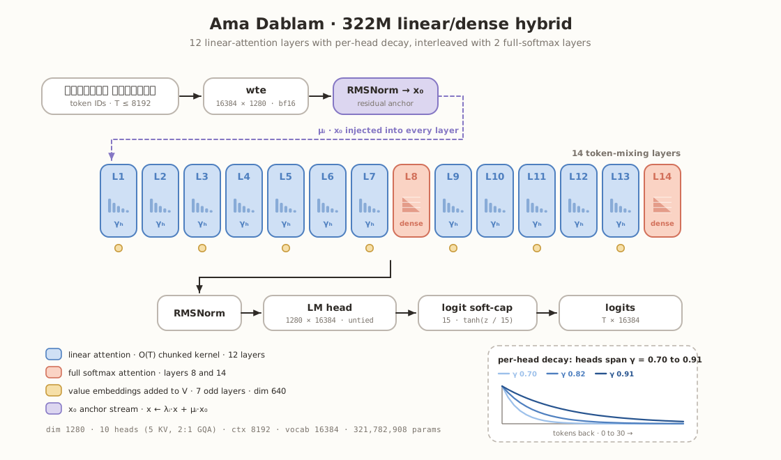
Inside one block (identical for linear and dense layers except the mixer):

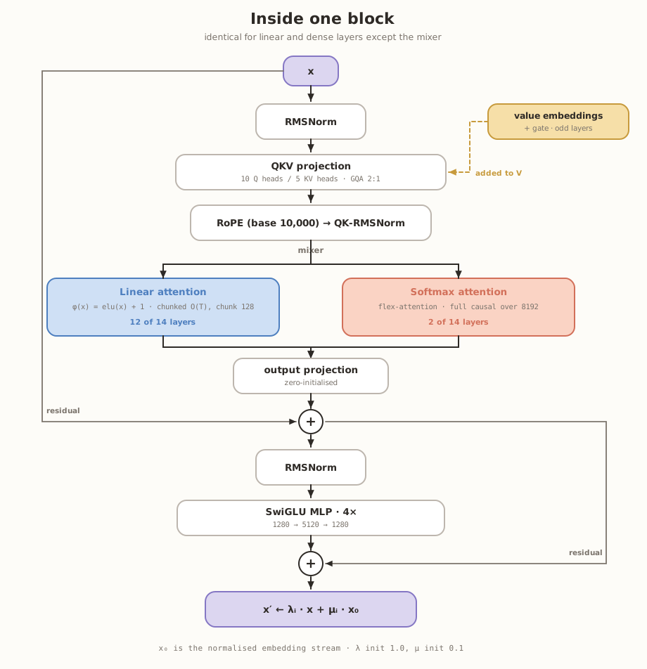
Parameter budget:

Component	Params
Token embedding (wte)	20,971,520
Value embeddings (7 layers)	73,400,320
LM head (untied)	20,971,520
Transformer matrices	206,439,520
Residual scalars	28
Total	321,782,908

4.2 Linear attention with per-head decay

Each linear layer computes causal, normalized linear attention with feature map \(\varphi(x) = \mathrm{elu}(x) + 1\) [8]:

\[\begin{aligned} \mathrm{out}_i &= \frac{\varphi(q_i)^{\top} S_i}{\varphi(q_i)^{\top} z_i} && \text{(normalized read)} \\[2pt] S_i &= \sum_{j \le i} \gamma^{\,i-j}\, \varphi(k_j)\, v_j^{\top} && \text{(decayed KV state)} \\[2pt] z_i &= \sum_{j \le i} \gamma^{\,i-j}\, \varphi(k_j) && \text{(decayed normalizer)} \end{aligned}\]

Why any decay is needed. The \(\gamma\) in those equations is not decoration; without it this layer does not work. Softmax attention compares every query against every key explicitly, which costs \(O(T^2)\) but lets any past token be retrieved at full resolution. Linear attention buys its \(O(T)\) cost by giving that up: the entire past is compressed into one fixed-size running state \(S \in \mathbb{R}^{D \times D}\), and whatever the model needs from earlier tokens must survive inside it. Set \(\gamma = 1\) and every token ever seen is added to that state with equal weight, so by a few thousand tokens the state is a sum of thousands of outer products in which any individual token contributes a vanishing fraction, and the read-out \(\varphi(q_i)^\top S_i\) returns a blur dominated by whatever is numerically largest rather than by what is relevant. The recency structure that language overwhelmingly depends on is simply absent. Decay fixes this in one multiplication: scaling the state by \(\gamma\) at each step weights a token \(j\) positions back by \(\gamma^{\,j}\), which builds in recency, bounds the effective number of tokens held in the state at roughly \(1/(1-\gamma)\), and stops the state from saturating no matter how long the sequence runs. Our own measurements say the same thing: at matched compute, the identical hybrid without decay sat near 0.82 bpb against 0.685 with it (§5), a gap far larger than any other architectural knob we swept.

Why the rate varies per head. A single global \(\gamma\) forces one compromise on the whole layer. A small \(\gamma\) gives sharp, strictly local mixing and forgets almost immediately; a large \(\gamma\) remembers longer but smears nearby tokens together, since the immediate neighbour and the token twenty back arrive at nearly equal weight. Attention heads specialize, so a layer benefits from having both available. We therefore give each head \(h\) its own rate, spaced by exponentiating the base LINEAR_DECAY = 0.7 (this is the RetNet mechanism [1]):

\[\gamma_h = 1 - (1 - 0.7)^{e_h}, \qquad e_h = \mathrm{linspace}(1, 2, H)\]

With \(H = 10\) heads this yields rates from \(\gamma_0 = 0.700\) to \(\gamma_9 = 0.910\). Writing the horizon as the half-life \(\ln 0.5 / \ln \gamma_h\), the tokens at which a head’s weighting has fallen by half:

head	0	1	2	3	4	5	6	7	8	9
\(\gamma_h\)	0.700	0.738	0.770	0.799	0.824	0.846	0.866	0.882	0.897	0.910
half-life (tokens)	1.9	2.3	2.7	3.1	3.6	4.2	4.8	5.5	6.4	7.3

The routing is learned rather than fixed: the rates are constants, but the Q/K/V projections decide what each head writes into and reads out of its state, so the model chooses per layer which horizon to exploit.

What this does and does not buy. The table is worth reading carefully, because it bounds the claim. Even the slowest head halves its weighting within about 7 tokens and retains only \(8 \times 10^{-5}\) of it 100 tokens back. These heads are local mixers: at this decay base the linear layers capture morphology, agreement, and short-range syntax, not document-level dependency. Long-range, content-based retrieval in this model is done entirely by the two dense softmax layers (§4.3), which is precisely why the hybrid keeps them rather than going fully linear. Choosing a decay base near 1 would extend the linear horizon, but our sweep found 0.7 optimal at probe scale (§5), and we did not re-sweep it at production scale or at the production context length: a limitation, given that the sweep ran at context 1,024 where long horizons cannot pay for themselves (§9).

Chunked O(T) kernel. Training uses a chunk-parallel formulation (chunk = 128): the within-chunk term is one batched matmul over all chunks under a causal mask with decay powers; only the inter-chunk state carry is sequential. The kernel is verified against a naive O(T²) reference to ~1e-7 in fp32. It is pure PyTorch, with no fused CUDA kernel, and the efficiency consequences are discussed in §6.4 and §9.

Reproducibility hazard: γ is derived from a module constant at construction time and is not stored in checkpoints. A loader that omits LINEAR_DECAY = 0.7 builds a decay-free model that loads the trained weights without any error and silently underperforms. Our SFT tooling pins the constant in a single loader module and verifies it by reproducing pretraining validation bpb before any fine-tuning (§8.4).

4.3 Dense layers

The two softmax layers use full causal attention over the entire 8,192-token context (flex-attention kernel under torch.compile during pretraining) with the same GQA layout. Interleaving occasional dense layers is the MiniMax-01-style hedge [18]: global, content-based retrieval where linear attention’s compressed state is insufficient.

4.4 Shared components

All layers share a common stack, identical to the 491M dense model’s:

• RoPE [19] (base 10,000, head-dim 128, precomputed to 10× context = 81,920 positions) followed by QK RMS-normalization [20].
• Value embeddings (the modded-nanogpt variant [33] of ResFormer-style value residuals [21]): 7 of 14 layers (alternating) add a learned per-token embedding (dim = KV width 640) to V, gated by 2·sigmoid(Linear(x[..., :32])) per KV head; gates initialize to zero.
• SwiGLU MLP [22] at 4× expansion: c_fc: 1280→5120, gate/value split, c_proj: 2560→1280.
• Per-layer residual scalars: x ← λ_i·x + μ_i·x₀ with λ init 1.0, μ init 0.1 (x₀ = the normalized embedding stream).
• Logit soft-capping [23] at 15 (15·tanh(logits/15)), untied LM head.
• Embeddings and value-embeddings held in bf16; matmul weights fp32 (bf16 autocast at compute).

4.5 Initialization

wte \(\sim \mathcal{N}(0, 1)\); LM head \(\sim \mathcal{N}(0, 0.001^{2})\); attention/MLP inputs uniform \(\pm\sqrt{3}\, d^{-1/2}\); all output projections zero-initialized; value-embedding gates zero-initialized (each layer starts as identity-plus-nothing and learns to open its gates).

---

5. Architecture Selection: Evidence and Caveats

The hybrid emerged from a tuning program at probe scale (depth 8 / dim 512 / ctx 1024). We report the positive and negative findings below.

Decay dominates. At equal compute (2.5×10¹⁵ FLOPs), val bpb traces a clean U in the decay base: 0.2→0.698, 0.4→0.692, 0.6→0.686, 0.7→0.685 (best), 0.8→0.689, 0.9→0.703, 0.95→0.737. Without decay the same hybrid sat near 0.82, so decay alone closed most of the gap to softmax.

Feature map choice is noise. relu² 0.8202 ≈ elu+1 0.8206 ≈ relu 0.8219 ≈ softplus 0.8237 at matched budget; we kept elu+1.

Learning-rate interaction. Enabling decay shifts the Muon-LR optimum down at probe token counts (flat valley ≈0.006–0.015 vs 0.05 without decay). We nevertheless trained production at matrix-LR 0.05, reasoning that the probe optimum is a data-starved artifact (the production run has ~100× the optimizer steps); this choice was not re-verified at production scale and is listed as a limitation.

The accounting trap (negative result). At equal FLOPs the hybrid beat all-dense by +0.008 bpb at 2.5×10¹⁵, but the margin shrank to ~0.003–0.004 (within single-seed noise) by 1×10¹⁶, and at equal tokens (≈ equal wall-clock under torch.compile, where per-token speeds matched) the tuned dense model won by ~0.004. Equal-FLOPs comparisons flatter linear attention at short context because its cheaper layers buy extra tokens that matter only in the data-starved regime. The small-scale evidence favored dense at ctx ≤ 8192 given current kernels. The hybrid was chosen as a bet on long-context asymptotics (O(T) attention, O(1) inference state). That bet is unsettled here, because no matched 322M dense baseline was trained at the production budget (2.84×10¹⁹ FLOPs). Comparisons to the earlier 491M dense model (§7) confound architecture with a 3.6× token budget and corpus differences.

Size selection. An IsoFLOP study on the earlier campaign’s corpus, following the Chinchilla methodology [25], fitted \(N^{*}(C) = 628\,C^{0.308}\) to three compute points (1.2, 2.4 and 4.8 × 10¹⁶ FLOPs, with compute-optimal sizes 58.5M, 63.6M and 89.6M).

Two caveats travel with this law, and we state them rather than lean on it silently. First, the exponent is loosely constrained: three points over a 4× span in compute support a band of roughly ±0.05–0.08, and the same measurements give 0.358 if \(N\) is counted without embedding tables, so part of the exponent is a bookkeeping choice. Because the three budgets are equally log-spaced, a fit through the two endpoints reproduces the three-point slope exactly, so that agreement is an algebraic identity rather than evidence of robustness; fits through adjacent pairs give 0.121 and 0.495. Second, 0.308 sits well below Chinchilla’s 0.5, which implies \(D^{*} \propto C^{0.692}\): in this setup extra compute is better spent on tokens than on parameters.

At the production compute the law suggests \(N^{*} \approx 600\text{M}\); we trained under it at 322M because the token target was set by data (1.5 epochs of the 11.4B-token corpus = 17.1B tokens, 53.1 tok/param) rather than by compute-optimality: a data-constrained, over-trained regime when the corpus, not compute, is the binding constraint. The same study fitted a loss curve \(L = E + A\,C^{-\alpha}\), but to three points, an exact fit that leaves the floor \(E\) unconstrained. Its extrapolation into this compute region (~0.40) is close to the achieved 0.4061 (§7.2), which we report as a directional check rather than a validated prediction.

---

6. Pretraining

6.1 Setup

Hardware	NVIDIA DGX Spark (GB10, Blackwell), 121 GB unified memory, CUDA 13.0
Framework	PyTorch nightly (cu130), bf16 autocast, torch.compile
Attention backend	flex-attention (dense layers); chunked PyTorch kernel (linear layers)
Seed	42
Global batch	2¹⁸ = 262,144 tokens/step (device micro-batch 8 × 8,192; grad-accum 4)
Token budget	17,100,000,000 (1.5 epochs; FLOPs budget 2.844×10¹⁹)
Steps	65,242

6.2 Optimizer: MuonAdamW

Two-dimensional transformer matrices are updated with Muon [26] (momentum-orthogonalized momentum; 5 Newton–Schulz/polar-express iterations, momentum 0.95 with a 300-step ramp from 0.85 and a −10% taper in the final 5% of training; second-moment β₂ 0.95; weight-decay 0.03 annealed as WD·(1−progress)). Everything else uses AdamW [27] (β = (0.85, 0.99), ε = 1e-10, no weight decay), with per-group learning rates scaled by (d_model/768)^−½ = 0.7746:

Group	Peak LR
Matrices (Muon)	0.05
Token embedding	0.3
Value embeddings	0.3
LM head	0.004
x₀ scalars	0.5 (β = (0.96, 0.95))
residual-λ scalars	0.005

Schedule: no warmup; LR multiplier = (1 − progress)/0.95 capped at 1.0, i.e., a linear warmdown to zero spanning 95% of training. This schedule shapes the loss curve (§6.3).

6.3 Training dynamics

Debiased-EMA train loss (bpb-scale surprise on the mixed corpus):

Step	0	100	1k	6k	12k	15k	20k	25k	30k	35k	52.6k	65,242
Loss	9.71	2.50	1.71	1.52	1.47	1.43	1.45	1.42	1.39	1.33	1.30	1.213

Two practitioner notes. First, the mid-run plateau (~steps 15k–25k) is a property of the schedule, not of learning: with LR still ≥ 0.6 of peak, the EMA sits in a 1.42–1.45 band before the warmdown’s back third unlocks a further −0.21 of loss. Second, the run stalled once (process death without traceback at step ~21,435, 3.3 days in) and was resumed from the step-20,000 checkpoint with full state restoration (model, optimizer, RNG, schedule position); the loss curve shows no discontinuity at the splice. Checkpoints carry {step, tokens_done, loss-EMA, timing, config, model, optimizer, RNG} every 5,000 steps.

6.4 Throughput and efficiency

Steady-state throughput was ~20,000 tokens/s (~13.1 s/step), for a total wall-clock of ≈10.2 days (2.84×10⁵ s pre-stall + 5.94×10⁵ s post-resume). Nominal MFU against an H100 bf16-peak denominator is 3.4%; this understates real utilization on GB10 hardware (different peak) but reflects the absence of a fused linear-attention kernel: the chunked pure-PyTorch path is the efficiency ceiling of this run, and equal-FLOPs accounting undercounts the hybrid’s true wall-clock cost relative to flash-attention baselines.

---

7. Pretraining Evaluation

7.1 Methodology

Bits per byte:

\[\mathrm{bpb} = \frac{\sum \text{nats}}{\ln 2 \cdot \sum \text{target-bytes}}\]

with zero-byte special tokens excluded from both sums. This is a tokenizer-agnostic quantity, enabling comparison across models, vocabularies, and scripts. Each validation shard is evaluated over ~21M tokens (sequence length 2,048), with the evaluation code held frozen across the entire campaign.

7.2 Results

Table: held-out bpb, Ama Dablam vs the earlier 491M dense model. (The 491M model’s IAST rows were computed under the earlier tokenizer; bpb’s byte normalization keeps the comparison valid.)

Metric	Earlier 491M dense	Ama Dablam 322M	Δ
ne (Devanagari, primary)	0.4324	0.4061	−6.1%
mai (Devanagari)	0.4383	0.3677	−16.1%
bho (Devanagari)	0.6320	0.5461	−13.6%
iast_ne (diagnostic)	0.3859	0.3258	−15.6%
iast_mai (diagnostic)	1.0220	0.7674	−24.9%
iast_bho (diagnostic)	1.3388	1.0317	−22.9%
phon_ne (diagnostic)	n/a	0.9422	first measurement

The campaign’s Nepali progression: 0.5380 (earlier Nepali-only run) → 0.4324 (491M dense) → 0.4061 (this work).

Attribution. The dominant driver is training volume, not architecture: Ama Dablam saw 3.6× the tokens (17.1B vs 4.8B) at 53 vs 9.8 tokens/parameter. The 491M dense model was knowledge-limited by design. That a 35%-smaller model surpasses it on every axis is the expected outcome of training past the data/compute lever (§10, item 3), and the outcome is close to what the earlier campaign’s IsoFLOP extrapolation suggested for this compute budget (~0.40 against 0.4061 achieved). We read that agreement as directional, not confirmatory, for the reason given in §5: the underlying loss fit has three points and an unconstrained floor. It should not be read as evidence that the hybrid architecture outperforms dense (§5).

Per-script observations. IAST improves more than Devanagari (−16 to −25%), reflecting the tokenizer’s larger romanized budget and the added IAST/phonetic corpus mass. The first phonetic-Nepali measurement (0.9422) is markedly harder than IAST-Nepali (0.3258): phonetic romanization is lossy (schwa deletion and retroflex/dental collapse destroy information a model must reconstruct from context), and phonetic text is only ~10% of the Nepali stream. Bhojpuri remains the weakest Devanagari language, consistent with its smallest and noisiest corpus.

---

8. Multi-Script Supervised Fine-Tuning

8.1 Objective and design principle

The SFT goal is instruction-following in all three scripts with continuity to pretraining, explicitly not teaching transliteration as a skill. Devanagari-only SFT (as in the earlier 491M model) would erode the base model’s romanized competence through catastrophic forgetting [2]; the design counters this in two places: multi-script instruction data and a replay stream matched to the pretraining mixture.

8.2 Dataset construction

Basis. The same four community Nepali instruction sources used for the earlier 491M model (machine/community-translated Alpaca–Dolly families [28, 29] plus Aya [30], comprising 4,002 human-annotated Aya-dataset and 4,002 templated Aya-collection records): multiturn 139,865 / alpaca-dolly-67k 67,017 / ibibek 49,601 / Aya 8,004 = 264,487 raw records. No new collection, no machine translation.

Multi-script partition. After normalization and a val-first 2% split, every example is assigned exactly one script by content hash (sha256 of its text → bucket in [0,100)): <85 Devanagari (unchanged), 85–89 rendered in IAST, 90–99 phonetically transliterated. The assignment is deterministic, order-independent, and disjoint (no parallel duplicates, since parallel data would constitute a transliteration-teaching signal, which is out of scope). The whole example moves together, with instruction, input, and output in the same script, so the model learns to reply in the script it is addressed in.

Rendering. Option A chat template over reserved tokens (⟨bos⟩⟨user⟩ instruction\ninput ⟨asst⟩ response ⟨eot⟩; ids 16368–16371), loss masked to response tokens through ⟨eot⟩ only, one example per sequence, cap 2,048 tokens.

Replay. 5% of the train-token volume (4.73M tokens; 2,310 rows of 2,049) sampled uniformly with a fixed seed from the 80 reshuffled pretraining shards. Because those shards already contain every language and script in trained proportions, uniform sampling reproduces the pretraining distribution with no mixing logic: the anchor matches what we are trying not to forget.

Realized dataset: 259,071 train / 5,288 val / 2,310 replay rows; script shares 0.8498 / 0.0501 / 0.1002 (target 0.85/0.05/0.10); 94.6M train tokens; 128 records dropped for over-length prompts, 0 for emptiness. Val carries the same script mix, enabling per-script response evaluation.

8.3 Training

Full fine-tune, identical to the 491M model’s recipe for attribution: AdamW (lr 1e-5, β = (0.9, 0.95), wd 0), cosine decay over all 48,576 steps, batch 16, 3 epochs, batch-level replay at 5%, gradient clip 1.0, bf16 autocast, eager execution, seed 7. Per-epoch self-describing checkpoints. Wall-clock: 8.7 h/epoch, ~26 h total (eager hybrid; most instruction sequences are far shorter than the 2,048 cap).

8.4 The loader gate (methodological contribution)

Because γ is not serialized (§4.2), we made the following protocol mandatory before any fine-tuning: the SFT loader must reproduce the base model’s pretraining validation metrics. The gate re-evaluated the loaded base checkpoint on all shards and required the four known values to match within ±0.005. Result: agreement to ≤0.00024 bpb on all four (ne 0.406064 vs 0.406123; mai 0.367742 vs 0.367698; bho 0.546068 vs 0.546059; iast_ne 0.325521 vs 0.325754), confirming the loader, the decay pinning, and fp32-eager numerical equivalence to the compiled bf16 training graph. The same check is useful wherever architectural constants live outside the checkpoint.

8.5 Results

Response-level bpb (loss over response tokens only, evaluated in chat format; “base” is the pretrained model prompted with the same template):

	base	epoch 1	epoch 2	epoch 3 (selected)	Δ base→e3
overall	0.5696	0.3594	0.3487	0.3471	−39.1%
Devanagari (n=4,529)	0.5236	0.3264	0.3164	0.3149	−39.9%
IAST (n=259)	1.0077	0.7167	0.6981	0.6955	−31.0%
phonetic (n=500)	1.1711	0.7637	0.7437	0.7410	−36.7%

(The IAST row rests on only 259 validation examples, the least precise of the three per-script estimates.)

Forgetting (drift vs the §8.4 baselines; gate ≤ +0.05):

Metric	e3 drift	Status
ne	+0.0107	OK
mai	+0.0301	OK
bho	+0.0387	OK
iast_ne	+0.0163	OK
phon_ne	+0.0302	OK
iast_mai	+0.0565	FLAG: accepted deviation
iast_bho	+0.0762	FLAG: accepted deviation

Every metric with replay/instruction coverage stays comfortably within the gate; the primary Nepali drift is a negligible +0.011. The two flagged metrics are precisely the combinations with zero instruction coverage and near-zero replay mass (IAST renderings of Maithili/Bhojpuri, which are diagnostics by design), and their drift is bounded and stable across epochs. Under the protocol’s human-adjudication clause, epoch 3 was selected: best response quality in every script at unchanged cost on all success metrics. We record explicitly that no epoch satisfied the strict all-seven gate.

Qualitative. On 20 pinned prompts (12 Devanagari / 4 phonetic / 4 IAST): 18/20 replied in the prompt’s script with coherent, on-instruction content, including IAST responses with correct diacritics and a five-city list that was more accurate in IAST than in Devanagari. Failure modes: the two creative Devanagari prompts (poem, birthday greeting) degenerated into English word-salad, for which residual English in the creative slices of the community SFT sources is the likely cause. Factual reliability remains that of a 322M model (Everest’s height was wrong in Devanagari and right in phonetic).

---

9. Discussion and Limitations

What this campaign establishes. Tokenizer fit, corpus curation, and token volume are enough to beat a larger undertrained baseline on these languages on a single workstation; romanized competence can be added via transliteration and kept via replay; a probe-scale IsoFLOP law picked a usable model-size region 592× beyond its fitting range, with its loss extrapolation agreeing to within 0.01 bpb on a single point.

What it does not establish.

1. Hybrid vs dense at scale remains open. No matched dense baseline exists at 2.84×10¹⁹ FLOPs; small-scale evidence at short context favored dense (§5). The hybrid’s intended advantage, long-context efficiency, was neither exercised (training ctx 8,192) nor kernel-supported.
2. Single-seed results. Every production number is one seed; probe-scale seed variance (~0.006 bpb) suggests the 491M-dense comparisons are far outside noise, but fine distinctions (e.g., epoch-2 vs epoch-3 SFT) are not.
3. Knowledge ceiling. 322M parameters and 17B tokens bound factual reliability; SFT demonstrably improved form (−39% response bpb) rather than facts.
4. Uncovered script–language pairs erode. IAST-mai/bho drifted +0.06–0.08 through SFT: the cost of zero coverage, and a clean quantitative illustration of the replay principle by its exception.
5. Evaluation breadth. bpb and a 20-prompt qualitative set; no downstream benchmark suite (IndicParam [4], FLORES [32]) has yet been run.
6. Phonetic transliteration is Nepali-tuned. Maithili/Bhojpuri text was romanized under Nepali schwa rules; dialectal fidelity is unquantified.

---

10. Practical Takeaways

Each item is tied to a measurement from this campaign.

1. Tokenizer first. A 16k domain-matched BPE achieves 0.47–0.49 tpc on Devanagari vs ~1.0 (cl100k) and ~1.6 (GPT-2), a 2–3× multiplier on effective context and compute before any modeling work. Budget vocabulary for the target languages, not for universality.
2. Use byte-normalized metrics. Every cross-script, cross-tokenizer, and cross-generation comparison in this report is only meaningful because bpb normalizes away the vocabulary.
3. Tokens beat parameters. 322M @ 53 tok/param surpassed 491M @ 9.8 tok/param on every metric with 35% fewer parameters. In the low-resource regime the corpus is usually the binding constraint, so spend effort growing and cleaning it, then train past the Chinchilla point [25] on what you have.
4. Sibling languages help. Trilingual training beat the Nepali-only baseline on Nepali (0.4324 vs 0.5380 for the earlier Nepali-only run), and gave Maithili and Bhojpuri models nearly for free; a shared script makes related languages mutually reinforcing rather than competitive.
5. Scripts can be added by transliteration. Deterministic IAST + phonetic rendering converted existing Devanagari data into romanized competence (iast_ne 0.326, phon_ne 0.942) at zero collection cost. For languages whose speakers type in Latin script, this is a capability native-script data alone does not provide.
6. Small scaling studies steer large runs, within limits. An IsoFLOP law fitted at ≤4.8×10¹⁶ FLOPs picked the model-size region for a run 592× larger, and its loss extrapolation (~0.40) landed near the achieved 0.4061. The size estimate is the more reliable half; the loss extrapolation rested on three points with no constrained floor (§5) and should be read as directional. A cheap scaling study is worth running before a long one, provided its error bars travel with it.
7. Replay in pretraining proportions limits forgetting. 5% replay held every covered metric to ≤ +0.04 drift through 3 SFT epochs, while the two zero-coverage combinations drifted +0.06–0.08.
8. Small models learn form, not facts. SFT cut response bpb 31–40% and produced reliable script-following, while factual errors persisted. Product plans for this model class should center formatting, extraction, and conversation, not QA.
9. Checkpoint reproducibility early. Self-describing checkpoints, full state resume (which saved this campaign at step 21,435), and loader gates for constants that live outside the checkpoint (γ) cost little and mattered here.
10. Prefer replay to bad machine translation. With no usable Bhojpuri MT, replay alone preserved Bhojpuri (+0.039) through Nepali-only instruction tuning.

---

11. Future Directions

Alignment and preference data. Ama Dablam is pretrained and instruction-tuned, but not aligned. SFT taught it the shape of a reply, and §8.5 shows that worked: response bpb fell 31–40% and the model answers in the script it is addressed in. SFT does not teach a model to choose between two replies that are both well formed, to decline a request, or to state that it does not know. Those behaviours are learned from preference data, meaning pairs of responses to one prompt with a human judgment of which is better, and we found no such dataset for Nepali, Maithili, or Bhojpuri. The open preference corpora are almost entirely English. The obstacle is the data rather than the method, since DPO and similar offline methods are inexpensive to run on a 322M model.

The same shortage already appeared one level down. Our SFT data was Nepali-only and mostly community- or machine-translated, and Maithili and Bhojpuri supplied no instruction data at all, which is why they appear in §8.5 only as forgetting metrics. Preference annotation is harder to source than instruction text, because it needs speakers who can compare two answers rather than write one.

Four steps, in the order we would take them:

1. Collect preference pairs from the model itself. Sample several responses per prompt from the instruct checkpoint and have Nepali speakers rank them. Responses drawn from the model being aligned are more useful per annotation than imported data, and offline preference optimization needs on the order of thousands of pairs rather than the 259,071 examples SFT consumed. The cost is annotator time, not GPU time.
2. Be wary of translated preference data. The caveats that applied to translated instruction data are stronger here. Which of two answers is better depends on register, politeness, and cultural fit, and translation can reverse the judgment. A mislabelled pair is worse than a missing one, because preference optimization will learn it.
3. Cover all three scripts. Devanagari-only alignment would erode romanized behaviour the way Devanagari-only SFT would have (§8.1). Preference data should carry the same script partition and the same 5% replay stream as §8.
4. Build the evaluation set first. Response bpb cannot measure helpfulness or refusal, and no automatic metric exists for these languages. A pinned set of prompts with native-speaker judgments, versioned like our validation shards, is a prerequisite for measuring whether alignment worked.

Grow the corpus where it binds. Bhojpuri and Maithili are data-limited: OCR of print archives, community text drives, and ASR transcripts are the highest-leverage additions per §10 item 3. For Nepali, targeted domain expansion (law, government, education) addresses the knowledge ceiling more than parameters will.

Instruction data beyond Nepali. Native mai/bho instruction collection first; Ne→Maithili machine translation (a short linguistic hop, supported by IndicTrans2 [31]) with round-trip filtering second; Bhojpuri MT when tooling matures.

SFT data hygiene. Strip English residue from creative-prompt slices (the observed degeneration mode); add explicit transliteration-skill tasks and cross-script instruction pairs (excluded here) as separate, controlled capabilities.

Benchmarks and community baselines. Run IndicParam [4] (Maithili) and FLORES-200 [32]; publish the first systematic Bhojpuri LM baselines; for these languages, evaluation infrastructure is itself a contribution.

Deployment. Deeper multi-turn training (the current model saw only flattened single-turn pairs); distillation and quantization toward phone-class inference, which matters here because most speakers of these languages reach a model through a phone.

Scale along the law. The next run this points to is roughly 900M parameters on about 18B tokens, which is where the size law of §5 lands at a compute budget of 10²⁰ FLOPs. Treat that as the centre of a sweep rather than a target: the law is being extrapolated some 2,000× beyond the largest budget it was fitted at, and carrying its exponent uncertainty through puts the plausible range nearer 550M to 1.5B.

The question worth answering at that budget is whether continued pretraining from Ama Dablam reaches the same quality as training from scratch. If it does, every later campaign starts from a checkpoint rather than from nothing.

---

12. Conclusion

Ama Dablam is a 322M-parameter linear/dense hybrid that reads and writes Nepali, Maithili, and Bhojpuri in Devanagari, IAST, and natural phonetic romanization. It was pretrained from scratch on 17.1B tokens on a single workstation over about ten days, then instruction-tuned to answer in whichever of the three scripts it is addressed in. On the pinned Devanagari validation shards it reaches 0.4061 bits per byte on Nepali, 0.3677 on Maithili, and 0.5461 on Bhojpuri. After multi-script instruction tuning, response-level bpb is 0.3471 overall, and on a pinned qualitative set the model replied in the prompt’s own script on 18 of 20 prompts.

The parts of the campaign that carried their weight were mostly unglamorous, and they are the parts we would repeat. A 16,384-entry tokenizer built for these languages spends 0.474 tokens per character of Nepali Devanagari against 1.031 for cl100k, a 2× multiplier on effective context and on compute per unit of text before any modelling decision is made. Exact-hash deduplication removed 4.2M documents from one source alone. A deterministic transliterator turned existing Devanagari text into a third writing system at no collection cost, which is how a model for languages with almost no romanized corpus came to read the Latin script its speakers actually type. A 5% replay stream drawn from the pretraining mixture held every script and language with instruction coverage to at most 0.04 bpb of drift across three epochs of fine-tuning, while the two combinations with no coverage drifted 0.057 and 0.076: the same principle appearing once as a result and once as its own exception.

The least supported part is the architecture. We chose a linear/dense hybrid as a bet on long-context efficiency, and that bet is unresolved here. No matched dense baseline was trained at this budget, the small-scale evidence we do have favoured dense at these context lengths, and at the decay base we actually trained the linear layers have half-lives under eight tokens (§4.2), so they act as local mixers while the long-range work falls to the two softmax layers. The advantage the hybrid was chosen for was never exercised at 8,192 tokens of context, and we would not repeat the choice without the matched baseline that would settle it.

Three limits bound what the model can be used for. Every production number comes from a single seed. At 322M parameters factual reliability stays poor, and instruction tuning improved the form of answers without repairing their content. And the model is not aligned, nor can it be until preference data exists for these languages, which at present it does not (§11). What the campaign does show is that for languages in this position the binding constraint is corpus and tokenizer fit rather than parameter count or architectural novelty, and that the equipment required is one workstation.

---

References

[1] Yutao Sun, Li Dong, Shaohan Huang, Shuming Ma, Yuqing Xia, Jilong Xue, Jianyong Wang, and Furu Wei. Retentive Network: A Successor to Transformer for Large Language Models. arXiv preprint arXiv:2307.08621, 2023.

[2] James Kirkpatrick, Razvan Pascanu, Neil Rabinowitz, Joel Veness, Guillaume Desjardins, Andrei A. Rusu, Kieran Milan, John Quan, Tiago Ramalho, Agnieszka Grabska-Barwinska, Demis Hassabis, Claudia Clopath, Dharshan Kumaran, and Raia Hadsell. Overcoming catastrophic forgetting in neural networks. Proceedings of the National Academy of Sciences, 114(13):3521–3526, 2017.

[3] David M. Eberhard, Gary F. Simons, and Charles D. Fennig (eds.). Ethnologue: Languages of the World. SIL International. Entries for Nepali (npi), Maithili (mai), and Bhojpuri (bho). https://www.ethnologue.com/

[4] Ayush Maheshwari, Kaushal Sharma, Vivek Patel, and Aditya Maheshwari. IndicParam: Benchmark to Evaluate LLMs on Low-Resource Indic Languages. arXiv preprint arXiv:2512.00333, 2025.

[5] Aleksandar Petrov, Emanuele La Malfa, Philip H. S. Torr, and Adel Bibi. Language Model Tokenizers Introduce Unfairness Between Languages. In Advances in Neural Information Processing Systems (NeurIPS), 2023. arXiv:2305.15425.

[6] Sneha Kudugunta, Isaac Caswell, Biao Zhang, Xavier Garcia, Derrick Xin, Aditya Kusupati, Romi Stella, Ankur Bapna, and Orhan Firat. MADLAD-400: A Multilingual And Document-Level Large Audited Dataset. arXiv preprint arXiv:2309.04662, 2023.

[7] Niraj Pahari and Kazutaka Shimada. Share What You Already Know: Cross-Language-Script Transfer and Alignment for Sentiment Detection in Code-Mixed Data. arXiv preprint arXiv:2402.04542, 2024.

[8] Angelos Katharopoulos, Apoorv Vyas, Nikolaos Pappas, and François Fleuret. Transformers are RNNs: Fast Autoregressive Transformers with Linear Attention. In International Conference on Machine Learning (ICML), 2020.

[9] Mohammed Safi Ur Rahman Khan, Priyam Mehta, Ananth Sankar, Umashankar Kumaravelan, Sumanth Doddapaneni, Suriyaprasaad G, Varun Balan G, Sparsh Jain, Anoop Kunchukuttan, Pratyush Kumar, Raj Dabre, and Mitesh M. Khapra. IndicLLMSuite: A Blueprint for Creating Pre-training and Fine-Tuning Datasets for Indian Languages. arXiv preprint arXiv:2403.06350, 2024. (Sangraha corpus.)

[10] Wikimedia Foundation. Wikipedia database dumps. https://dumps.wikimedia.org/

[11] The International Alphabet of Sanskrit Transliteration (IAST), standardized by the Transliteration Committee of the Tenth International Congress of Orientalists, Geneva, 1894; as used in Monier Monier-Williams, A Sanskrit-English Dictionary, Oxford University Press, 1899. (ISO 15919:2001 is the closely aligned modern ISO standard.)

[12] Jayaraj Acharya. A Descriptive Grammar of Nepali and an Analyzed Corpus. Georgetown University Press, 1991.

[13] Rajesh Khatiwada. Nepali. Journal of the International Phonetic Association, 39(3):373–380, 2009. (See also standard treatments of schwa deletion in Indo-Aryan orthography.)

[14] Rico Sennrich, Barry Haddow, and Alexandra Birch. Neural Machine Translation of Rare Words with Subword Units. In Proceedings of ACL, 2016.

[15] Alec Radford, Jeffrey Wu, Rewon Child, David Luan, Dario Amodei, and Ilya Sutskever. Language Models are Unsupervised Multitask Learners. OpenAI technical report, 2019. (GPT-2 byte-level BPE.)

[16] OpenAI. GPT-4 Technical Report. arXiv preprint arXiv:2303.08774, 2023. (cl100k / tiktoken-style BPE split conventions.)

[17] Ashish Vaswani, Noam Shazeer, Niki Parmar, Jakob Uszkoreit, Llion Jones, Aidan N. Gomez, Łukasz Kaiser, and Illia Polosukhin. Attention Is All You Need. In Advances in Neural Information Processing Systems (NeurIPS), 2017.

[18] MiniMax, Aonian Li, Bangwei Gong, et al. MiniMax-01: Scaling Foundation Models with Lightning Attention. arXiv preprint arXiv:2501.08313, 2025.

[19] Jianlin Su, Yu Lu, Shengfeng Pan, Ahmed Murtadha, Bo Wen, and Yunfeng Liu. RoFormer: Enhanced Transformer with Rotary Position Embedding. arXiv preprint arXiv:2104.09864, 2021.

[20] Biao Zhang and Rico Sennrich. Root Mean Square Layer Normalization. In Advances in Neural Information Processing Systems (NeurIPS), 2019. arXiv:1910.07467.

[21] Zhanchao Zhou, Tianyi Wu, Zhiyun Jiang, Fares Obeid, and Zhenzhong Lan. Value Residual Learning. arXiv preprint arXiv:2410.17897, 2024. (ResFormer.)

[22] Noam Shazeer. GLU Variants Improve Transformer. arXiv preprint arXiv:2002.05202, 2020. (SwiGLU.)

[23] Gemma Team, Morgane Riviere, Shreya Pathak, et al. Gemma 2: Improving Open Language Models at a Practical Size. arXiv preprint arXiv:2408.00118, 2024. (Logit soft-capping.)

[24] Joshua Ainslie, James Lee-Thorp, Michiel de Jong, Yury Zemlyanskiy, Federico Lebrón, and Sumit Sanghai. GQA: Training Generalized Multi-Query Transformer Models from Multi-Head Checkpoints. arXiv preprint arXiv:2305.13245, 2023.

[25] Jordan Hoffmann, Sebastian Borgeaud, Arthur Mensch, Elena Buchatskaya, Trevor Cai, Eliza Rutherford, Diego de Las Casas, Lisa Anne Hendricks, Johannes Welbl, Aidan Clark, Tom Hennigan, Eric Noland, Katie Millican, George van den Driessche, Bogdan Damoc, Aurelia Guy, Simon Osindero, Karen Simonyan, Erich Elsen, Jack W. Rae, Oriol Vinyals, and Laurent Sifre. Training Compute-Optimal Large Language Models. arXiv preprint arXiv:2203.15556, 2022. (Chinchilla / IsoFLOP.)

[26] Keller Jordan, Yuchen Jin, Vlado Boza, Jiacheng You, Franz Cesista, Laker Newhouse, and Jeremy Bernstein. Muon: An Optimizer for Hidden Layers in Neural Networks. 2024. https://kellerjordan.github.io/posts/muon/

[27] Ilya Loshchilov and Frank Hutter. Decoupled Weight Decay Regularization. In International Conference on Learning Representations (ICLR), 2019.

[28] Rohan Taori, Ishaan Gulrajani, Tianyi Zhang, Yann Dubois, Xuechen Li, Carlos Guestrin, Percy Liang, and Tatsunori B. Hashimoto. Stanford Alpaca: An Instruction-Following LLaMA Model. 2023. https://github.com/tatsu-lab/stanford_alpaca

[29] Mike Conover, Matt Hayes, Ankit Mathur, Jianwei Xie, Jun Wan, Sam Shah, Ali Ghodsi, Patrick Wendell, Matei Zaharia, and Reynold Xin. Free Dolly: Introducing the World’s First Truly Open Instruction-Tuned LLM. Databricks blog, 2023.

[30] Ahmet Üstün, Viraat Aryabumi, Zheng-Xin Yong, Wei-Yin Ko, Daniel D’souza, Gbemileke Onilude, Neel Bhandari, Shivalika Singh, Hui-Lee Ooi, Amr Kayid, Freddie Vargus, Phil Blunsom, Shayne Longpre, Niklas Muennighoff, Marzieh Fadaee, Julia Kreutzer, and Sara Hooker. Aya Dataset: An Open-Access Collection for Multilingual Instruction Tuning. arXiv preprint arXiv:2402.06619, 2024.

[31] Jay Gala, Pranjal A. Chitale, Raghavan AK, Varun Gumma, Sumanth Doddapaneni, Aswanth Kumar M, Janki Nawale, Anupama Sujatha, Ratish Puduppully, Vivek Raghavan, Pratyush Kumar, Mitesh M. Khapra, Raj Dabre, and Anoop Kunchukuttan. IndicTrans2: Towards High-Quality and Accessible Machine Translation Models for All 22 Scheduled Indian Languages. Transactions on Machine Learning Research, 2023. arXiv:2305.16307.

[32] NLLB Team, Marta R. Costa-jussà, James Cross, Onur Çelebi, Maha Elbayad, Kenneth Heafield, Kevin Heffernan, Elahe Kalbassi, Janice Lam, Daniel Licht, Jean Maillard, Anna Sun, Skyler Wang, Guillaume Wenzek, Al Youngblood, Bapi Akula, Loic Barrault, Gabriel Mejia Gonzalez, Prangthip Hansanti, John Hoffman, Semarley Jarrett, Kaushik Ram Sadagopan, Dirk Rowe, Shannon Spruit, Chau Tran, Pierre Andrews, Necip Fazil Ayan, Shruti Bhosale, Sergey Edunov, Angela Fan, Cynthia Gao, Vedanuj Goswami, Francisco Guzmán, Philipp Koehn, Alexandre Mourachko, Christophe Ropers, Safiyyah Saleem, Holger Schwenk, and Jeff Wang. No Language Left Behind: Scaling Human-Centered Machine Translation. arXiv preprint arXiv:2207.04672, 2022. (FLORES-200.)

[33] Keller Jordan and contributors. modded-nanogpt: NanoGPT speedrun. GitHub repository, 2024. https://github.com/KellerJordan/modded-nanogpt (Origin of the gated value-embedding variant, the x₀ residual scalars, and the Muon training recipe adopted here.)

---

Appendix A: Reproducibility

Code map (two repositories):

Artifact	Location
Pretraining trainer + dense model	autoresearch/version2_pretrain_inference.py
Hybrid model + chunked kernel	autoresearch/version2_linear_pretrain_inference.py
Production launcher	autoresearch/train_300m_hybrid.py
Corpus pipeline	trilingual-lm-specs/setup_trilingual_data.py, integrate_extra_sources.py, generate_phonetic_shards.py, reshuffle_train_shards.py
Transliterators	trilingual-lm-specs/transliterate_iast.py, transliterate_phonetic.py (+ gold tests)
Round-2 tokenizer	trilingual-lm-specs/build_round2_tokenizer.py
Data/tokenizer/eval library	trilingual-lm-specs/prepare_trilingual.py (frozen through the campaign)
SFT dataset builder	trilingual-lm-specs/sft/build_multiscript_sft.py
SFT trainer / evaluator / loader / generation	trilingual-lm-specs/sft/{train,eval}_sft_amadablam.py, sft/amadablam_model.py, sft/generate_amadablam.py

Seeds: pretraining 42; corpus phonetic sampling 1234; SFT split 7; SFT script assignment: content-hash (seedless, deterministic); replay sampler 20260713; SFT training 7.

Checkpoints: base ckpt_0065243.pt (2.47 GB; step 65,242); SFT amadablam_sft_e{1,2,3}.pt (1.29 GB each); selected: e3 (recorded with baselines in sft_data/amadablam_baselines.json).

Wall-clock: pretraining ≈ 10.2 days (incl. one stall/resume at step 21,435); SFT 26 h; loader-gate baseline eval 2.3 h; per-epoch eval ~2.3 h.

Known follow-ups (tracked in the project ledger): fused linear-attention kernel; strict missing-key assertion in the SFT loader; drift-boundary test at exactly +0.05; stale special-token test from the earlier tokenizer; SFT resume does not restore optimizer moments (crash-recovery only).

Appendix B: The Chunked Linear-Attention Kernel

For queries/keys/values \(Q, K, V \in \mathbb{R}^{B \times H \times T \times D}\), feature map \(\varphi = \mathrm{elu} + 1\), chunk size \(c = 128\), per-head decay \(\gamma_h\):

Within each chunk of length \(c\), the causal term is computed directly with a masked matmul carrying decay powers \(\gamma^{\,i-j}\) for \(j \le i\) inside the chunk. Between chunks, a state \(S \in \mathbb{R}^{D \times D}\) and normalizer \(z \in \mathbb{R}^{D}\) are carried with per-chunk decay \(\gamma^{c}\):

\[\begin{aligned} S_{n+1} &= \gamma^{c} S_n + \sum_{t \in \text{chunk } n} \gamma^{\,c-t}\, \varphi(k_t)\, v_t^{\top} \\[2pt] z_{n+1} &= \gamma^{c} z_n + \sum_{t \in \text{chunk } n} \gamma^{\,c-t}\, \varphi(k_t) \\[4pt] \mathrm{out}_i &= \frac{\varphi(q_i)^{\top} \left( \gamma^{\,i \bmod c} S_n \right) + \text{within-chunk}_i} {\varphi(q_i)^{\top} \left( \gamma^{\,i \bmod c} z_n \right) + \text{within-norm}_i} \end{aligned}\]

The within-chunk term is one batched matmul over all chunks (vectorized); only the S/z carry is sequential. The kernel matches an O(T²) reference to ~10⁻⁷ (fp32) and its prefix-state formulation is what enables O(1)-memory inference in principle; realizing that in practice requires the fused kernel listed under future work.

Appendix C: Corpus Acceptance Checks

Executed before pretraining: tokenizer round-trips on all three languages and both romanizations; pinned val shards byte-stable (06542 byte-identical to the earlier campaign’s shard); Devanagari share 0.947 (target 0.94 ± 20%); phonetic val leak check (source-disjointness of sakonii from phonetic training inputs); post-reshuffle document counts reconcile with pre-reshuffle inputs; dataloader determinism under fixed seed.

Appendix D: SFT Dataset Acceptance Checks

Script shares within ±1% of 85/5/10 on train and val (realized .8498/.0501/.1002); record counts reconcile (264,487 raw = 259,071 train + 5,288 val + 128 truncation drops); template round-trip (tokenize→decode identity, incl. IAST diacritics); loss-mask offsets exact on all three scripts; the earlier model’s prior SFT shards byte-identical before/after the build (md5); 20+20 manual inspection of IAST/phonetic renderings; residual Devanagari in IAST slice 0.023% of characters (rare codepoints outside the mapping: nukta, candra-o).

Appendix E: The 491M Dense Baseline

Our earlier 491M-parameter dense model is internal and unpublished; trained earlier in this campaign, it is the measured baseline throughout this report. The facts needed to interpret every comparison:

	Earlier 491M dense
Parameters	490,735,136 (~491M)
Architecture	Decoder-only, all-softmax (dense) attention (SDPA)
Layers / model dim	16 / 1,536
Heads	12 (head dim 128), 6 KV heads (2:1 GQA)
Context length	2,048
Vocabulary	16,384 (its own tokenizer; same size and training-recipe family as Ama Dablam’s)
Shared stack	Same as §4.4: RoPE + QK RMS-norm, gated value embeddings, SwiGLU 4×, per-layer residual scalars, logit soft-capping, untied head
Optimizer	MuonAdamW (same family as §6.2)
Token budget	4,791,728,748 (~4.8B; 9.8 tok/param), cosine LR to zero
FLOPs budget	1.23 × 10¹⁹
Corpus	The §2.1 base trilingual corpus (Devanagari + IAST), before the phonetic and extra-source additions of §2.3–2.4
SFT	Devanagari-only instruction tuning over the same four sources as §8.2

Evaluation used the identical frozen bpb code (§7.1) on the identical pinned validation shards (§2.5); bpb’s byte normalization keeps all cross-tokenizer comparisons valid. Differences from Ama Dablam beyond architecture (3.6× fewer tokens, shorter context, a different tokenizer, no phonetic corpus) are why §7.2 attributes the headline gap to training volume rather than architecture.