Makalu - Decision Model

Makalu is a decision model with 0.6B parameters. It gives a score to each option of a decision. It also gives a probability that shows how sure it is. Makalu does four tasks:

It finds the correct passage for a question.
It gives a probability to each answer of a multiple-choice question.
It selects the next action for an agent.
It estimates if a finished coding attempt will pass its tests.

This post describes the final architecture and the three training phases: pre-training, mid-training and post-training. It also gives the results on each benchmark.

Agents that use large language models (LLMs) make many small decisions. A call to a large model for each decision is slow and expensive. A “System One” model is a small model that scores these decisions quickly. It reads the situation one time and each option one time. Then it scores all options in one pass.

We use the method of the Contrastive Language Models (CLM) project. CLM pre-trains on question–passage pairs and post-trains on agent data. Makalu is approximately 13 times smaller than the CLM model. Thus, each stage can run on one desktop GPU.

At a glance: each stage on its own task

Stage	Task	Before	After
Pre-training	retrieval, top-1 over 21,600 passages	0.770	0.809
Mid-training	multiple choice, test accuracy	0.280	0.592
Post-training 1	agent next action, val accuracy	0.468	0.706
Post-training 2	verification, SWE-bench best-of-4	0.602 (random pick)	0.732

1. Final architecture

Makalu starts from the Qwen3-Embedding-0.6B encoder. We add one low-rank adapter (LoRA) in the encoder. We also add two small scoring rules on top of the encoder. The 0.6B base weights do not change in any stage (they are frozen). We train only three parts: the adapter, a sharpness parameter \(\alpha\) and the verifier head.

Text goes through the frozen Qwen3 encoder. LoRA adapters are in all 28 layers. The encoder pools the last token and applies L2 normalisation. The unit vector goes to the choice scorer or to the verifier head. — **Figure 1: The Makalu decision model.** The same encoder does all tasks. The encoder uses left padding and pools the text at its last token. For a decision with options, the encoder encodes the state and each option separately. Cosine similarity compares the state with each option. A learned sharpness α scales these scores. A softmax changes the scores into one probability for each option. For a finished coding attempt, a linear head reads the embedding e of the attempt. The head gives P(pass). Questions and states have an instruction prefix. Options and passages do not have a prefix.

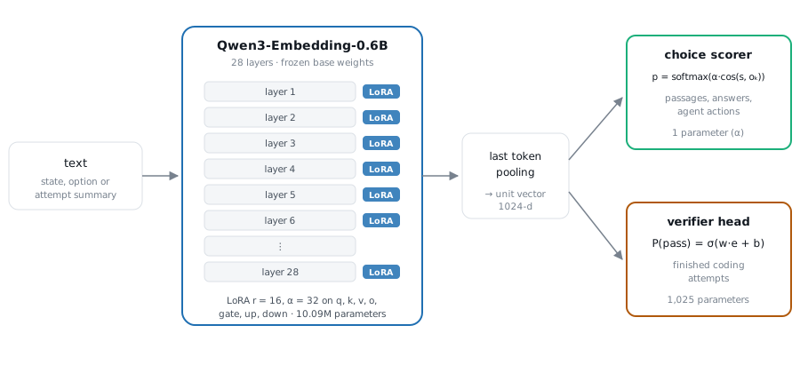
Table 1. What is trained

Part	Parameters	Trained in
Qwen3-Embedding-0.6B base	~596M	frozen in all stages
LoRA adapter (28 layers × 7 projections)	10.09M	every stage
Sharpness α (choice scorer)	1	mid- and post-training
Verifier head w, b	1,025	post-training 2

The trainable part is 1.7% of the parameters of Makalu. We also tested a 6.3M-parameter MLP projection head from our earlier retrieval experiments. We put this head on top of the LoRA model. Its results were equal or worse on each benchmark. Thus, Makalu does not have a projection head.

2. Methodology

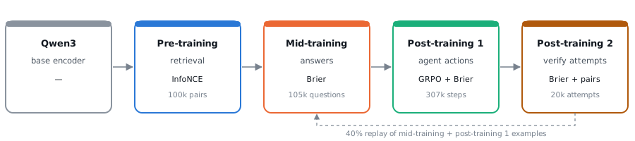
We train the same adapter in three phases: pre-training, mid-training and post-training. Post-training has two steps. Each stage starts from the checkpoint of the previous stage. Each stage trains a more difficult decision.

Mid-training and post-training use a Brier loss. This loss is the squared difference between the predicted probability and the true result. With this loss, the model gets a reward when it ranks the correct option first. It also gets a reward when its probabilities agree with how frequently it is correct.

Qwen3 to pre-training, mid-training, post-training 1 and post-training 2, with the task and loss of each step. — **Figure 2: The training pipeline.** Each box is one training step. The box shows the task, the loss and the size of the training set. The arrows show that the LoRA adapter goes to the next step. In post-training 2, 40% of the steps also use examples from mid-training and post-training 1 again (replay). Replay keeps these skills.

Pre-training: retrieval

We pre-train the adapter on question–passage pairs from PAQ and StackExchange. Each batch has 64 questions. We score each question against all 64 correct passages. We also score it against one mined hard negative for each question. A hard negative is an incorrect passage that is similar to the correct passage. The loss is InfoNCE. InfoNCE is the cross-entropy of the selection of the correct passage:

\[\mathcal{L} = -\log \frac{\exp\!\big(20\cdot\cos(q, d^{+})\big)}{\sum_j \exp\!\big(20\cdot\cos(q, d_j)\big)}\]

Mid-training: probabilities over answers

Each multiple-choice question becomes one state and four options. The state is the question with the instruction prefix. We encode each option together with its question (“Question: … Answer: …”). Thus, the model can examine the answer in the context of the question.

We train on OpenBookQA and MMLU with the Brier loss. This loss is the squared distance between the predicted probabilities \(p\) and the correct answer \(y\). The value of \(y\) is 1 for the correct option and 0 for the other options:

\[\mathcal{L} = \sum_k (p_k - y_k)^2, \qquad p = \operatorname{softmax}\big(\alpha \cdot \cos(s, o_k)\big)\]

Post-training 1: choosing an agent’s next action

We use 198,296 recorded agent trajectories from 23 datasets. The datasets include web browsing, household tasks, databases, terminals and software engineering. We change each trajectory into a sequence of decisions. At each step, the state is the task and the recent history. The options are the action that the agent did and three actions from other steps.

We train with GRPO, a policy-gradient method. The model samples 8 choices for each state. Each choice gets this reward:

\[r = y - (q - y)^2\]

In this equation, \(y\) is 1 if the sampled action is the logged action, and 0 if not. The value \(q\) is the confidence that the model gives for the action. The first term gives a reward for the correct action. The second term is a Brier penalty on confidence.

The confidence has its own temperature, and only the Brier term trains this temperature. If the confidence does not have a separate temperature, the reward causes the model to give full confidence for each choice. A KL penalty (\(\beta = 0.02\)) keeps the policy near the mid-trained model.

Post-training 2: verifying finished coding attempts

Several coding agents try the same task. The verifier reads each attempt, and the system submits the attempt with the highest score. We make each attempt into a summary of a maximum of 2,048 tokens. Each field of the summary has a fixed token budget (Figure 3).

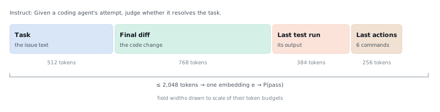
Fields of an attempt summary and their token budgets: task 512, final diff 768, last test run 384, last actions 256. The maximum total is 2,048 tokens. — **Figure 3: An attempt summary.** The task field keeps the first 384 tokens and the last 128 tokens of the task. The diff shows source edits first and scratch files after them. The test output comes from the last command that ran tests. The model encodes a summary one time. Thus, one forward pass gives the score for one attempt.

The loss has three parts:

Brier loss on P(pass). This part gives calibrated probabilities.
Ranking loss on hard-negative pairs. Each pair has one passing attempt and one failing attempt from the same task. The failing attempt is the attempt that the model gave the highest score. This part trains the model to separate attempts that are similar.
Replay loss. This part is the Brier loss of mid-training and post-training 1. It applies on 40% of the steps.

\[\mathcal{L} = \big(\sigma(w \cdot e + b + o_a) - y\big)^2 + \operatorname{softplus}\big(-(s_{\text{pass}} - s_{\text{fail}})\big) + \mathcal{L}_{\text{replay}}\]

The term \(o_a\) is a fixed offset. It is the log-odds of the pass rate of the agent in training. In the SWE-bench data, the agents pass between 10% and 76% of the time. Without the offset, the model can get a good score if it identifies the agent that wrote an attempt. With the offset, the head gets credit only for the information in the content of the attempt. At test time, we remove the offset. Thus, Makalu scores only the content.

3. Training

All stages ran on one GPU with 128 GB of unified memory. Each run was in a process with a memory limit, and gradient checkpointing was on. The full pipeline took approximately 39 GPU hours.

Table 2. Training setup per stage

Stage	Training data	Loss	Batch	LR	Steps	Hours
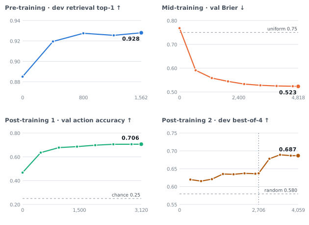
Pre-training	100k PAQ + StackExchange pairs	InfoNCE + hard neg.	64	1e-4	1,562	11.0
Mid-training	105,440 questions (OBQA, MMLU)	Brier	16	2e-5	4,818	8.0
Post-training 1	306,965 steps, 23 agent datasets	GRPO, Brier reward	16 × 8	1e-5	3,120	7.6
Post-training 2 (a)	20,273 attempts, 2,154 tasks + replay	Brier + agent offset	8	1e-5	2,706	8.0
Post-training 2 (b)	same + 10,152 hard-negative pairs	+ pair ranking	8	1e-5	1,353	4.1

The learning rates in Table 2 are for the LoRA adapter. The learning rate for α is 1e-2. The learning rate for the verifier head is 1e-3. Each schedule is a cosine decay with a 5% warm-up. We used only held-out dev or validation splits for model selection. We scored each test set one time only.

Four training curves on held-out data. Pre-training dev retrieval top-1 increases from 0.885 to 0.928. Mid-training val Brier decreases from 0.768 to 0.523. Post-training 1 val action accuracy increases from 0.468 to 0.706. Post-training 2 dev best-of-4 increases from approximately 0.62 to 0.687. It jumps after we add the hard-negative pairs at step 2,706. — **Figure 4: Training curves on held-out data.** Each panel starts at the starting checkpoint of its stage. Retrieval dev: 2,000 questions and 21,600 passages. Mid-training val: OBQA and MMLU validation sets. Post-training 1 val: 21 agent datasets, each with a minimum of 50 validation steps. Post-training 2 dev: 81 held-out tasks and 1,949 attempts. The dashed line shows the step where we added the hard-negative pairs.

4. Results

Figure 5 compares the model after each stage with the checkpoint at the start of that stage. The comparison uses the held-out test of the stage. Each stage improved its own task. The smallest gain is +0.04 on retrieval. The largest gain is +0.31 on multiple choice.

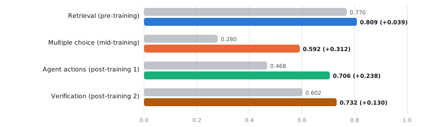
Before and after each stage: retrieval 0.770 to 0.809, multiple choice 0.280 to 0.592, agent actions 0.468 to 0.706, verification 0.602 to 0.732. — **Figure 5: Each stage on its own task.** Grey bars show the starting checkpoint. Coloured bars show the result after the stage. **Retrieval:** top-1 accuracy, 2,000 test questions against 21,600 passages (p = 2×10⁻¹²). **Multiple choice:** test accuracy on 7,520 questions with 4 options. Chance is 0.25. **Agent actions:** validation accuracy with 4 options. Chance is 0.25. **Verification:** SWE-bench Verified test. The metric is the pass rate of the attempt that the model selects from 4 attempts. The starting point is a random selection.

Makalu on every benchmark

Makalu keeps the three decision skills, and its probabilities stay calibrated. But Makalu loses part of its retrieval accuracy. Retrieval is the only skill that post-training did not replay.

Table 3. Makalu against the base encoder

Benchmark	Metric	Qwen3 base encoder	Makalu	Reference
Retrieval (21,600 passages)	top-1 ↑	0.770	0.650	after pre-training 0.809
Multiple choice (OBQA + MMLU val)	accuracy ↑	0.283	0.587	chance 0.25
	Brier ↓	0.751	0.542	uniform 0.75
Agent next action (21 datasets, val)	accuracy ↑	0.400	0.714	chance 0.25
	Brier ↓	0.687	0.379
SWE-bench Verified (95 tasks, test)	best-of-4 ↑	0.664	0.732	random 0.602 · perfect 0.874
	AUROC ↑	0.59	0.739	guessing 0.5
	calibration error ↓	—	0.050
Terminal-Bench 2.1 (89 tasks, test)	best-of-2 ↑	—	0.618	random 0.601 · perfect 0.787

“Best-of-N” is the pass rate of the attempt that the model selects from N attempts at the same task. We calculate the exact average over all subsets of N attempts. For the base encoder, we measured SWE-bench on the same 95 tasks with the zero-shot pipeline (full trajectories, 2,264 attempts). For Makalu, we used the attempt summaries (2,272 attempts). We did not use Terminal-Bench for training.

Table 4. Skills along the pipeline (every checkpoint scored on every task)

Checkpoint	Retrieval top-1 ↑	MC Brier ↓	MC accuracy ↑	Agent accuracy ↑	Agent Brier ↓
Qwen3 base	0.770	0.751	0.283	0.400	0.687
after pre-training	0.809	0.768	0.285	0.421	0.666
after mid-training	0.703	0.523	0.581	0.468	0.643
after post-training 1	0.727	0.547	0.566	0.706	0.391
Makalu (after post-training 2)	0.650	0.542	0.587	0.714	0.379

The multiple-choice and agent-action skills stay stable after the model learns them. Retrieval is highest after pre-training. It decreases in the stages that do not train on it.

Selection of the passing attempt

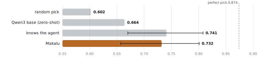
SWE-bench Verified test, best-of-4 pass rate: random pick 0.602, Qwen3 base zero-shot 0.664, knows-the-agent baseline 0.741 (95% CI 0.670–0.808), Makalu 0.732 (95% CI 0.657–0.801); perfect pick 0.874. — **Figure 6: SWE-bench Verified test, best-of-4 pass rate with 95% intervals.** We calculated the intervals with a bootstrap that resamples tasks. The "knows the agent" line is a baseline that does not read the attempt. It ranks attempts by the pass rate of their agent in training. Makalu reads only the content, and its result is equal to the baseline (0.732 and 0.741, and the intervals overlap). For attempts from one agent, the agent identity cannot help. In this case, the AUROC of Makalu is 0.672, and the AUROC of the baseline is 0.5.

These results have three limits:

Most runs used one seed. The dev and test sets for verification are small (81 and 95 tasks). Thus, differences of less than approximately 0.01 are in the noise.
Terminal-Bench has only 2 attempts for each task. Thus, it is a weak test of selection.
The backbone has only 0.6B parameters. CLM found that a larger encoder gave the largest gains. We did not test a larger encoder.

All numbers are on held-out data. We used only dev and validation splits for model selection. We scored each test set one time only.